Bayesian Theorem and Naive Bayes Classifier

Some uncertain events like whether the Arctic Ice Cap will disappear completely by the end of the century, cannot be repeated numerous time in order to define the notion of probability.
For such an event, we generally have some idea such as we may think that the ice cap is melting at the rate of 100,000 square kilometers each year. But from the fresh observation of earth via satellite we found out that the rate of ice loss is more than 200,000 square kilometers every year. Such new evidence affects our opinions on uncertain events. So it is necessary to revise uncertainty in the light of new evidence we just found. This can be done using the Bayesian interpretation of Probability.
Introduction to Bayesian Theorem
The fundamental idea behind all Bayesian Statistic is Bayesian Theorem. So it is vital to understand what is Bayesian Theorem.
Bayes' Theorem answers the questions "based on the data(or predictors) we have observed, what is the probability that the outcome is class \(C_L\). Mathematically, If \(\mathbf{Y = Class Variable}\) and \(\mathbf{X}\) represents the collection of predictor variables, and we are trying to estimate \(P[Y=C_L \hspace{0.6em}|\hspace{0.6em} X]\), i.e what is the probability that the outcome falls on the \(L^{th}\) class given \(\mathbf{X}\) is true, it is given as \[P[Y=C_L\hspace{0.6em} | \hspace{0.6em}X] = \frac{{P[Y] \hspace{0.6em}P[X\hspace{0.6em}|\hspace{0.6em}Y = C_L]}}{{P[X]}}\] P[Y] = Probability of the Y being true(regardless of the data). It is the prior probability.$$\\$$ P[X] = Probability of predictor values.$$\\$$ \(P[X\hspace{0.6em}|\hspace{0.6em}Y=C_L]\) is conditional probability of observing predictor values(or data) given class is \(C_L\).$$\\$$Bayes Theorem for Naive Bayes Classifier
In a classification problem, say we got a vector \(\mathbf{X}\) representing \(\mathbf{N}\) features as \(X{\rm{ }} = {\rm{ }}\left[ {x_1,{\rm{ }}x_2,{\rm{ }}x_3,{\rm{ }}...{\rm{ }},{\rm{ }}x_N} \right]\) and we got L classes \(C_1, C_2, C_3, .., C_N\) The main aim of the Naive Bayes algorithm is to find the probability that the class is \(\mathbf{C_k}\) given that the features are X. The Naive Bayes algorithm makes the use of Bayes Theorem which is given as \[P[C_k\hspace{0.6em} | \hspace{0.6em}X] = \frac{{P[C_k] \hspace{0.6em}P[X\hspace{0.6em}|\hspace{0.6em}C_k]}}{{P[X]}}\]In the above formula, the denominator P[X] is only a normalizing term which allows us to calculate the probability. Since it is constant and is only used to normalize we can drop it. So, by the defination of the conditional probability the RHS of given equation becomes
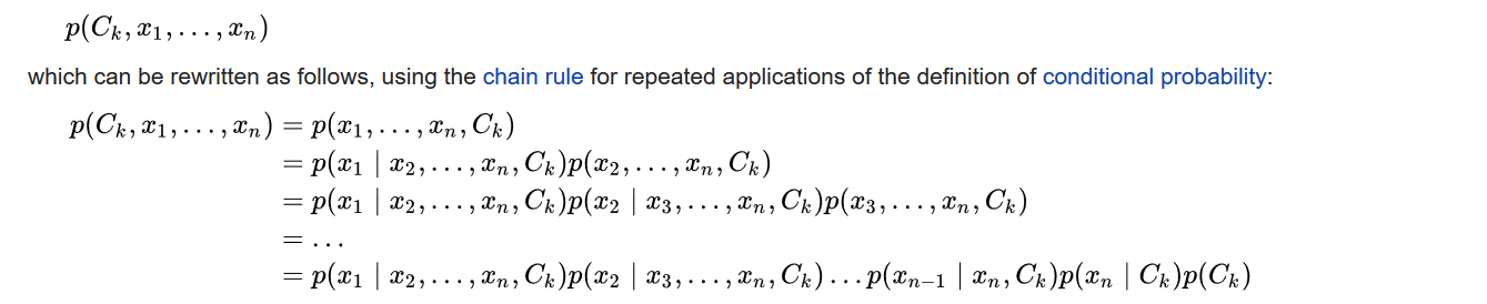
Now the Naive comes to play:
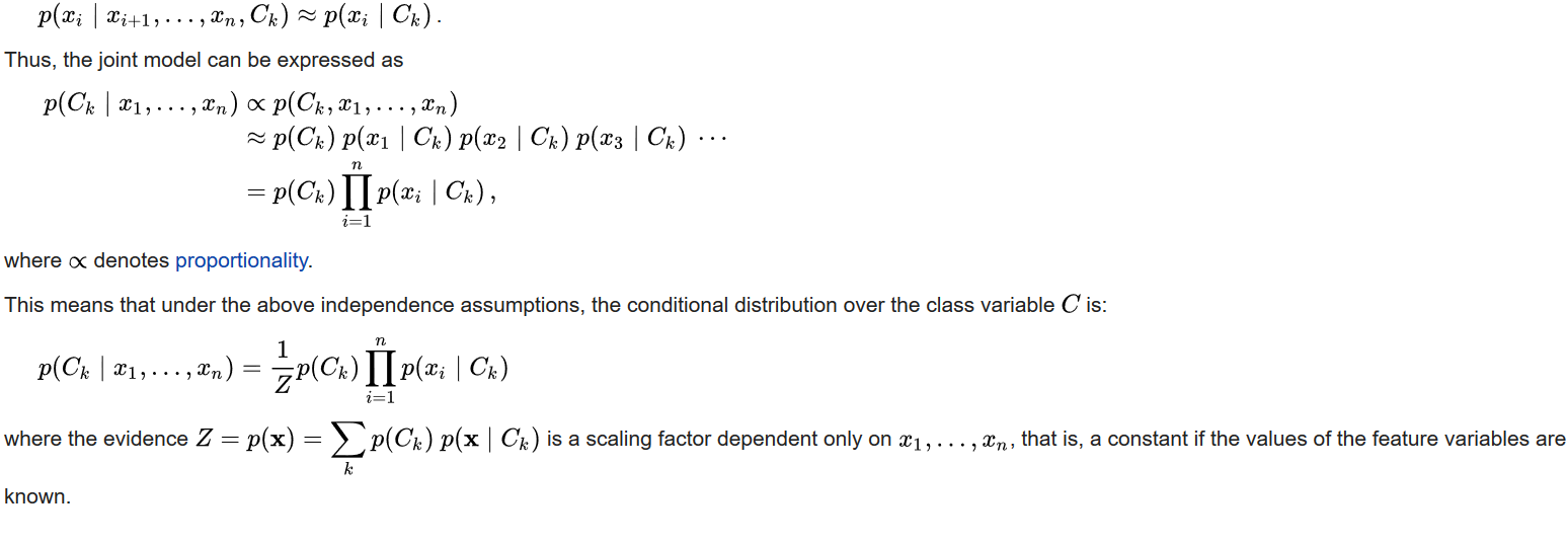
The above equation is good but will require a lot of computational power. So we make assumptions to simplify it. We make a assumption that features in X are conditionally independent of other feature of X.
If the features are conditionally independent with each other then we can write,