Simple Linear Regression Tutorial
Linear Regression attempts to model the relationship between two variables by fitting a linear equation to observed data.
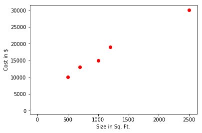
Say we got following data of housing industry,
\[\begin{array}{*{20}{c}} \hline {House Size(Sq.Ft.)}&\ {Cost(US\$ )}\\ \hline {500}& {10,000} \\ \hline {700}& {13,000} \\ \hline {1000}& {15,000} \\ \hline {1200}& {19,000} \\ \hline {2500}& {30,000} \\ \hline \end{array}\]Now, based on the data provide, we need to find the cost of the house of size 2000 Sq. Ft. For that, we will first plot the data.
In Linear Regression, what we try to do is fit our observed data by best possible linear equation(in this case it is a straight line) and next, we will predict the outcome for the unknown as shown in the image below.
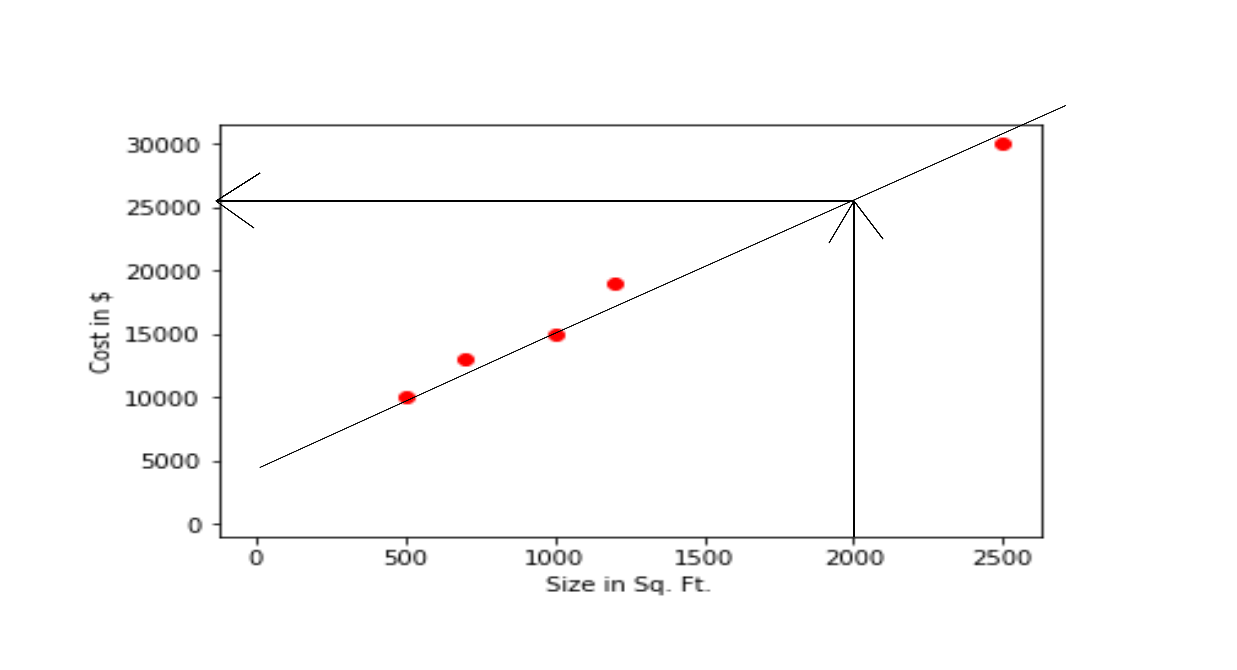
By seeing the above image we can find that the price of the house will be $25,300.
What is a Linear Regression?
Linear regression is a linear approximation of a causal relationship between two or more variables. Linear Regression is a linear model, e.g a model that assumes a linear relationship between the input variables(X) and the single output variable(Y).
The output(Y) can be calculated from a linear combination of the input variables(X). When there is a single input variable it is called as the Simple Linear Regression and when there is more than one input variable then it is referred to as the Multiple Linear Regression.
When using regression analysis we want to predict the value of (Y) provided we have a value of X and Y must depend on X in some casual way, whenever there is a change in X, the change must be translated in Y.
Representation of Linear Regression
Linear Regression is represented as linear equation that combines a specific set of input values(X) to give predicted value(Y).
The linear equation assigns one scale factor to each input value(\(X\)), that is commonly represented by the Greek Letter Beta(\(\beta\)). One additional coefficient is also added, giving the line an additon degree of freedom. Simple linear regression is represented as:
$$Y \approx \beta_0 + \beta_1X$$\(\beta_0\) and \(\beta_1\) are two unknown constants that represents \(intercept\) and \(slope\) terms in the linear model. Together \(\beta_0\) and \(\beta_1\) are known as model \(coefficients\) or \(parameters\). The higher the value of the coefficient higher the influence is. So if the value of the coefficient is 0, then the particular input variable will have no influence at all. We use the training data to estimate the value of \(\beta_0\) and \(\beta_1\) and make a predictions with it.
Loss Function for Regression
Loss function is a method of evaluating the correctness of specific algorithm which models the given data. If the prediction deviates too much from the actual results, loss function will be very high.
Loss function is quite straight forward in classification as L(h, (X,Y)) simply indicates whether h(x) correctly predicts or not.
In regression, if the weight of person is 60kg, both the prediction of 60.00001kg and 61kg are wrong. But we would surely prefer the prediction of 60.00001kg instead of 61kg. So we need a mechanism to penalized the discrepancy between estimated value and actual result.
One common way is to use the Square-Loss Function.
For a single data point,
\[L(h,(x,y)) = ((h(x) - Y)^2\]for all the data points,
\[Ls(h,(x,y)) = \sum\limits_{i = 1}^m {(h(x_i) - Y_i)^2} \]To make math easy, The \(\frac{1}{{m}}\) is to average the squared error over number of components so that the number of components doesn't affect the function and the \(\frac{1}{{2}}\) doesn't matter at all as minimizing L will also minizmize 2L.
\[Ls(h,(x,y)) = \frac{1}{{2m}}\sum\limits_{i = 1}^m {(h(x_i) - Y_i)^2} \] \(h(x_i)\) = Our prediction\(Y_i\) = Actual result
m = size of training data
Goal = Minimize the loss function
Using Gradient Descent to minimize the loss function
Imagine we are at any point of a mountain. In gradient descent, what are we going to do is spin 360 degree around and find the direction in which we have to make a baby step in order to go down the mountain as rapidly as possible.
After the finding that direction, we will make a baby step. Now we are in the another position in the mountain. Here we will repeat the previous step that is we will spin 360 degree around and find the direction of steepest descent. We will continue this preocess until we are at the lowermost portion of the mountain NG (2021).
Bibliography
Andrew NG. Machine Learning by Stanford University. url: https://www.coursera.org/learn/machine-learning/lecture/8SpIM/gradient-descent , 2021. [Online; accessed 5-July-2020]. ↩